Writing My Own PPO Implementation and Making It Fast
Getting my own PPO implementation correct, profiling it, and benchmarking it against the four RL libraries bundled with Isaac Lab.
I wrote my own implementation of PPO rather than using one off the shelf. Why? I wanted to understand how this algorithm works, as it is the state of the art for RL control in robotics, and very similar to the algorithms used for fine-tuning of LLMs. The next question is how does my implementation compare to existing ones? Isaac Lab ships with four established RL libraries, so this is a question I can actually answer rather than argue about. This post covers the two things I had to do before I could answer it, which were making the implementation correct, and then making it fast.
My implementation of PPO can be found here.
Making it right
My implementation already worked across a number of Gymnasium environments, including Atari Pong, but the Isaac Lab tasks are considerably harder and they exposed three problems with my implementation.
Weight initialization I was already using orthogonal initialization, which I had found out I drastically improved performance on the Atari environments, but I had missed that the output layer needs a different gain from the rest of the network, 0.01 for the actor and 1 for the critic.
No adaptive learning rate I was initially using a constant learning rate, and a decaying learning rate during training. I found during my research that adaptive learning rate schedulers are also used, which increase or decrease the learning rate based on the KL values for a specific update.
Observation normalization I had been using min/max normalization on my observations, but this requires an observation space that is bounded. These environments do not have defined bounds for every observation, such as object positions or goal positions. I switched to a running mean and variance estimator, using the Welford’s algorithm implementation which other libraries also use, as it is an efficient method of calculating the running mean and std deviation of the distribution.
Making it fast
Once it was learning reliably I decided to look into the performance of the code with profilers. Through this, I was able to get a grasp of what portions of the code were taking up the most execution time, and what portions of the code I could actually improve the efficiency of. Due tot he fact that the physics simulation was a large portion of the execution time, and these libraries were shipped with Isaac Lab, I did not expect that I would be able to make my implementation significantly faster than the provided ones. I was wrong on this, as many of these implementations decided on giving up small performance gains that ‘improved’ readability, which added up.
Sampling actions during training Sampling actions with torch.distributions.Normal turned out to be roughly 14 times slower than writing the Gaussian log probability out by hand. This gets called once per environment step, so it dominated the per-iteration overhead.
A single synchronization point I was calling .item() on the KL divergence once per minibatch, which forces a GPU to CPU synchronization and stalls the pipeline on every update. This was one of my first times really using and profiling code that is running on a GPU, so I learned a lot about limiting synchronization between the CPU and GPU.
Compiling functions into CUDA graphs This is easy to do, with simple PyTorch @torch.compile function decorators. I compiled the normalization updates, adaptive learning rate updates, the action selection, the critic value calculation, the GAE computation, and the mini-batch loss computation. One thing that I did not notice immediately was the benefit of minibatch indexing inside the loss function, instead of inside the arguments when calling the loss function. When indexing in the arguments at the call site, the indexing was not captured in the compilation. This allowed the indexing to become part of the captured graph rather than host side work being replayed around it.
Staggered episodes By default I start all my episodes at the start of an episode. This can result in a few quirks with my implementation. First, I log my data once based on the rollout that just finished. When a task has no terminal states, and only truncates, this results in a jagged staircase effect in the plotted results. Another quirk is that in this case each environment is in lockstep with each other, and each rollout only updates the network with data from a specific portion of an episode. To fix this, I first tried initializing every episode at a random step within an episode. This caused a drastic slowdown in my implementation, caused by the same issue of no terminal states. This meant that every step of every rollout a subset of environments needed to reset themselves, causing a slowdown on every step. To fix this, I instead start each environment at quantized intervals equal to the rollout length. This way, for a task with non-terminal states the reset cost is only paid once per rollout, while still providing smooth recording and data from various portions of the episode within each rollout.
Data types Initially the parameters of my model were all FP32. At one point I tried enabling TF32 activations, but then my training started to fail and I incorrectly attributed issues that surfaced as a result of the change to the change itself. I am still using FP32/TF32 for my networks, but I have done some experimentation using BF16 for activations. This improved the performance significantly, but I found that the policy itself was not the best, likely due to the reduced precision, which the robot needs to use specific encoder steps.
Smaller things Switching the optimizer to a fused implementation, and moving my own timing instrumentation onto CUDA events, so that measuring the code no longer serialized it. These are small changes, but when combined with my other changes, they add up.
Benchmarking against the bundled libraries
I benchmarked this implementation against the four RL libraries bundled with Isaac Lab — rsl_rl, rl_games, skrl, and sb3 on three tasks, cartpole, ant, and my SO-ARM101 reach task. Every run used 8,192 parallel environments on an RTX 5080, headless, and each library’s agent config matched. This is a throughput speed measurement, however my library has a slightly longer startup due to pytorch compilation of some functions. In a short run like cartpole, this could effect the total time more significantly than longer runs. I think with the speedup that they provide, especially for more complex tasks that require long runs, the benefits outweigh this penalty.
Cartpole — 16 steps/env
| Framework | Throughput (steps/s) | Iteration (ms) | Update (ms) | ryan_ppo speedup |
| ryan_ppo (this repo) | 1,816,704 | 72 | 5 | — |
| skrl | 1,183,419 | 111 | 34 | 1.54× |
| rl_games | 1,173,036 | 112 | 31 | 1.55× |
| rsl_rl | 1,136,048 | 115 | 35 | 1.60× |
| sb3 | 694,571 | 189 | — | 2.62× |
Ant — 32 steps/env
| Framework | Throughput (steps/s) | Iteration (ms) | Update (ms) | ryan_ppo speedup |
| ryan_ppo (this repo) | 994,079 | 264 | 27 | — |
| skrl | 893,478 | 293 | 54 | 1.11× |
| rl_games | 885,594 | 296 | 49 | 1.12× |
| rsl_rl | 832,319 | 315 | 56 | 1.19× |
| sb3 | 508,995 | 515 | — | 1.95× |
Reach — 24 steps/env
| Framework | Throughput (steps/s) | Iteration (ms) | Update (ms) | ryan_ppo speedup |
| ryan_ppo (this repo) | 1,947,558 | 101 | 16 | — |
| skrl | 946,503 | 208 | 119 | 2.06× |
| rl_games | 880,621 | 223 | 127 | 2.21× |
| rsl_rl | 657,378 | 299 | 139 | 2.96× |
| sb3 | 546,775 | 360 | — | 3.56× |
ryan_ppo has the highest throughput on every task: 1.11–2.06× the next-fastest library and 2.0–3.6× sb3. For every task, the execution time for the physics is largely unchanged library to library, and the library implementation controls the interface of the agent with the physics, and the update steps of the PPO algorithm. My library has a sigificantly faster update portion, and some of the surrounding framework for the rollouts is also optimized better.
Faster environments
I also worked on improving the performance of the task itself, to see how far I could get it. There are a few areas that help with this. First, using a direct workflow instead of a manager based workflow in isaaclab removes the overhead that the managers add for the actions, observations, and rewards. Additionally, the functions used for the actions, observations, and rewards can also be optimized to reduce execution time and GPU->CPU syncs. Lastly, the use of the Newton physics backend also results in a performance gain. This backend is based on Mujoco MJWarp, built ontop of NVIDIA’s Warp library, which provides fast GPU accelerated physics. As you can see below, the Cartpole and Ant tasks are using the shipped direct Newton workflows for those tasks, which provide a significant speedup, as well as my reach task, using a similar method, also provides a drastic speedup.
Cartpole (direct, Newton) — 16 steps/env
| Framework | Throughput (steps/s) | Iteration (ms) | Update (ms) | ryan_ppo speedup |
|---|---|---|---|---|
| ryan_ppo (this repo) | 3,508,178 | 37 | 4 | — |
| skrl | 1,739,236 | 75 | 34 | 2.02× |
| rl_games | 1,654,663 | 79 | 34 | 2.12× |
| rsl_rl | 1,636,259 | 80 | 36 | 2.14× |
| sb3 | 845,351 | 155 | — | 4.15× |
Ant (direct, Newton) — 32 steps/env
| Framework | Throughput (steps/s) | Iteration (ms) | Update (ms) | ryan_ppo speedup |
|---|---|---|---|---|
| ryan_ppo (this repo) | 2,097,027 | 125 | 27 | — |
| skrl | 1,522,399 | 172 | 54 | 1.38× |
| rl_games | 1,494,115 | 175 | 50 | 1.40× |
| rsl_rl | 1,325,754 | 198 | 57 | 1.58× |
| sb3 | 648,647 | 404 | — | 3.23× |
Reach (direct, Newton) — 24 steps/env
| Framework | Throughput (steps/s) | Iteration (ms) | Update (ms) | ryan_ppo speedup |
|---|---|---|---|---|
| ryan_ppo (this repo) | 2,880,358 | 68 | 16 | — |
| skrl | 1,106,186 | 178 | 118 | 2.60× |
| rl_games | 1,062,657 | 185 | 126 | 2.71× |
| sb3 | 620,027 | 317 | — | 4.65× |
| rsl_rl | 503,670 | 390 | 145 | 5.72× |
What else I have trained with it
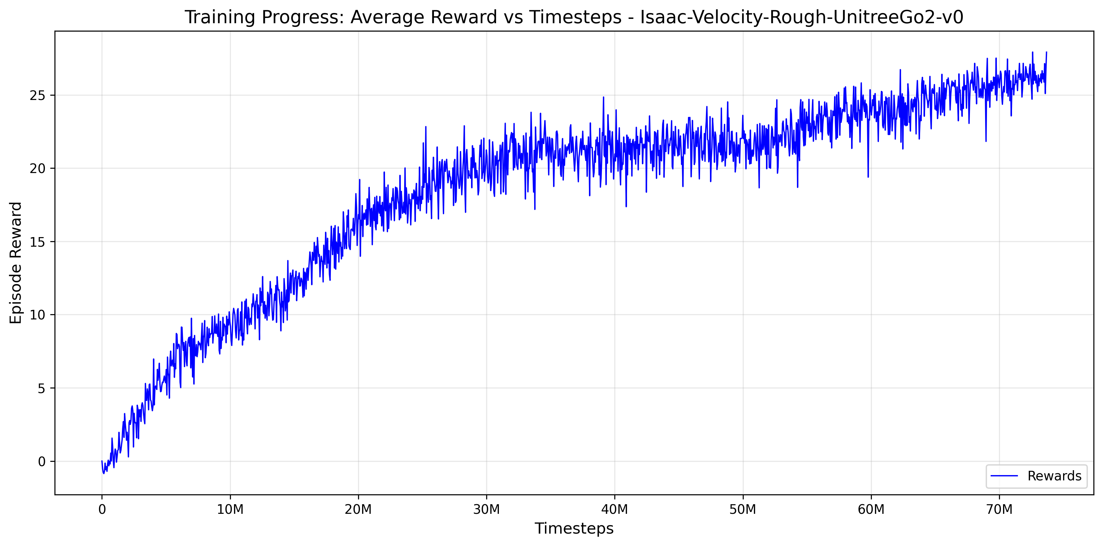
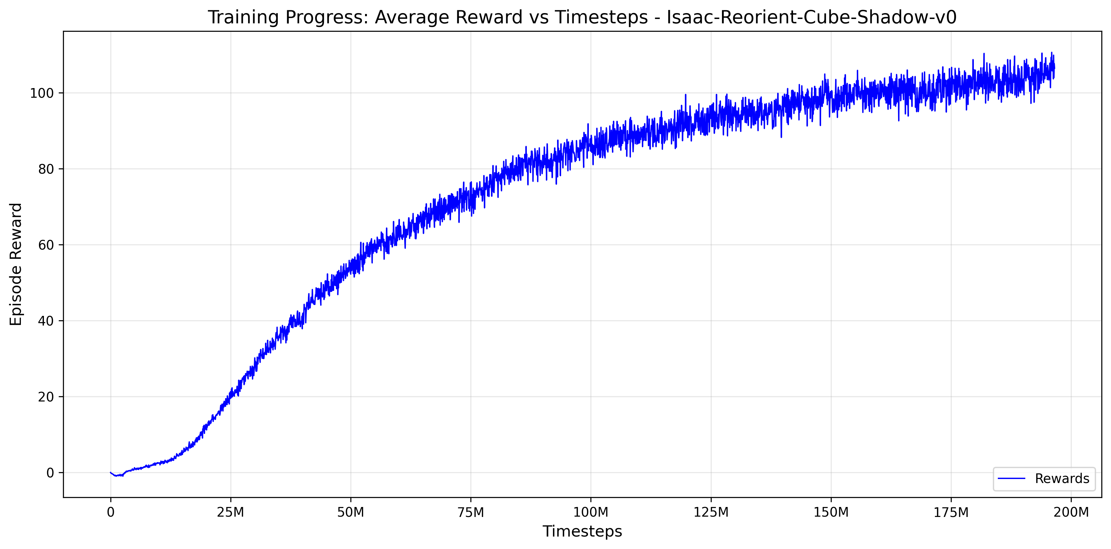
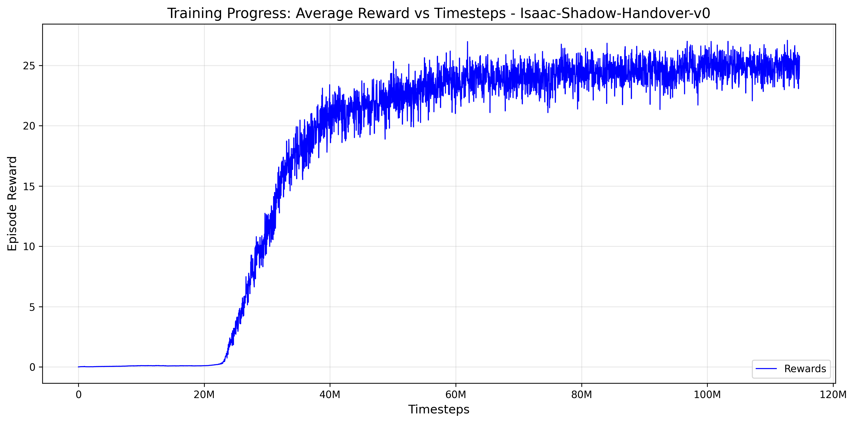
The plots below show the training progress across the range of Isaac Lab environments I have used this implementation on:
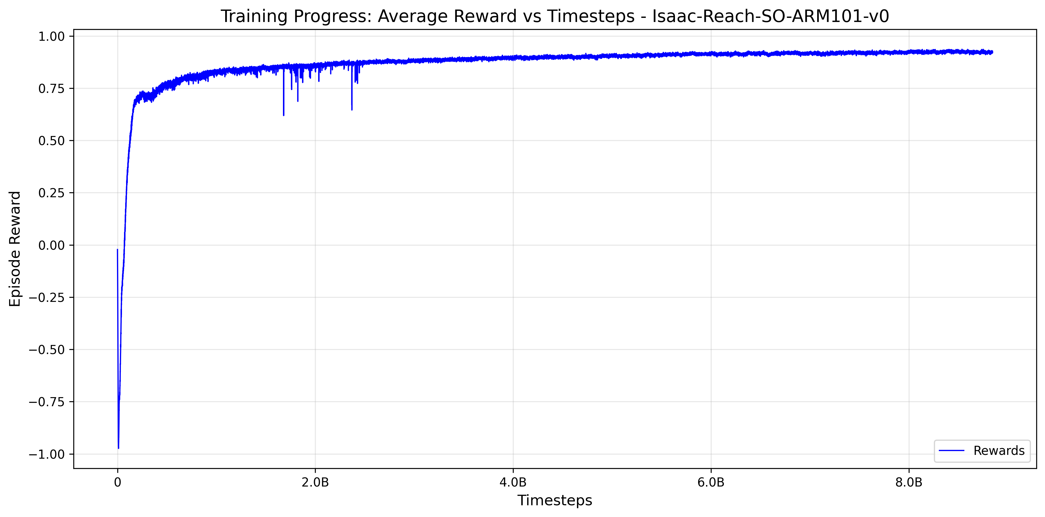
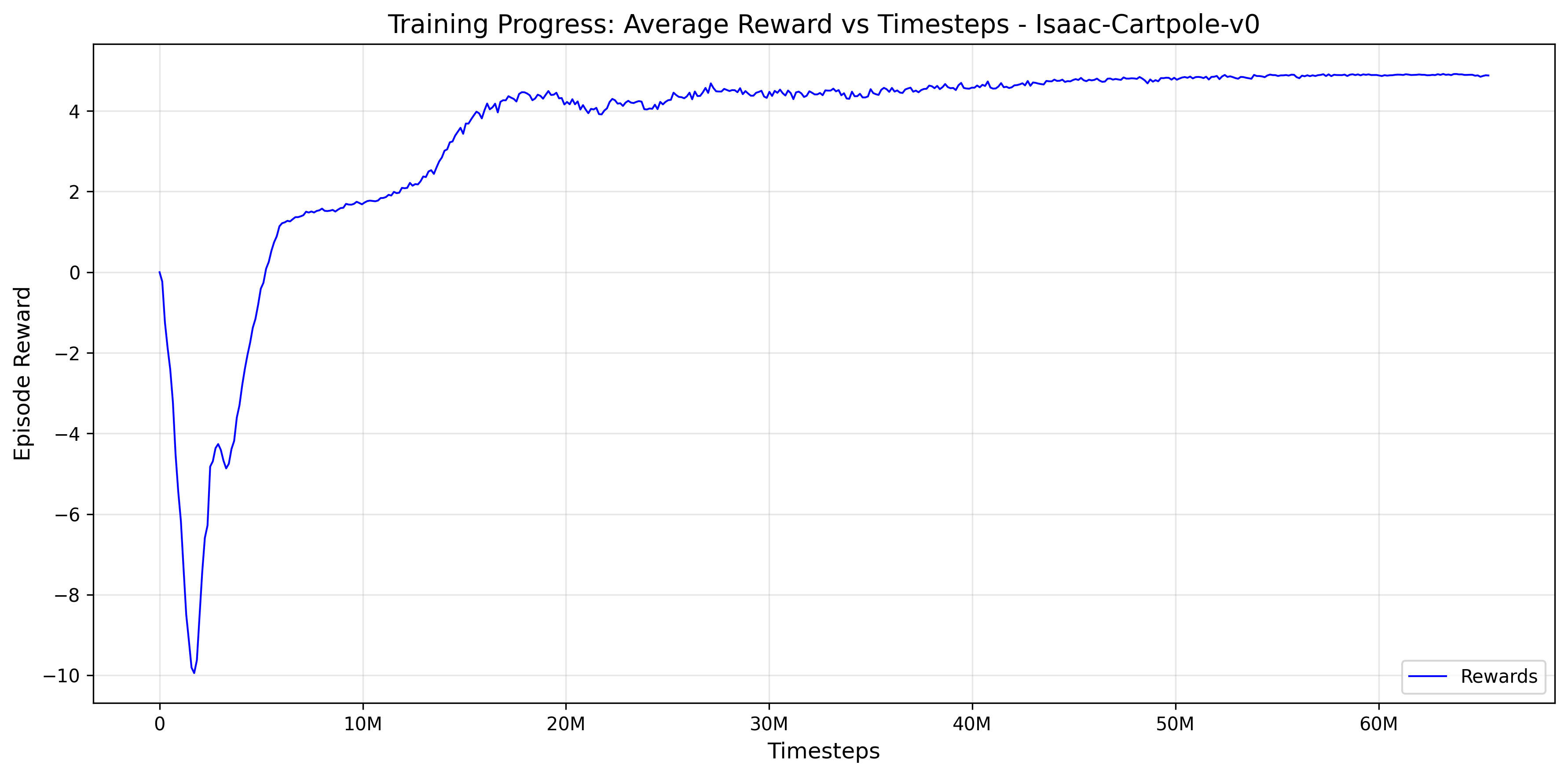
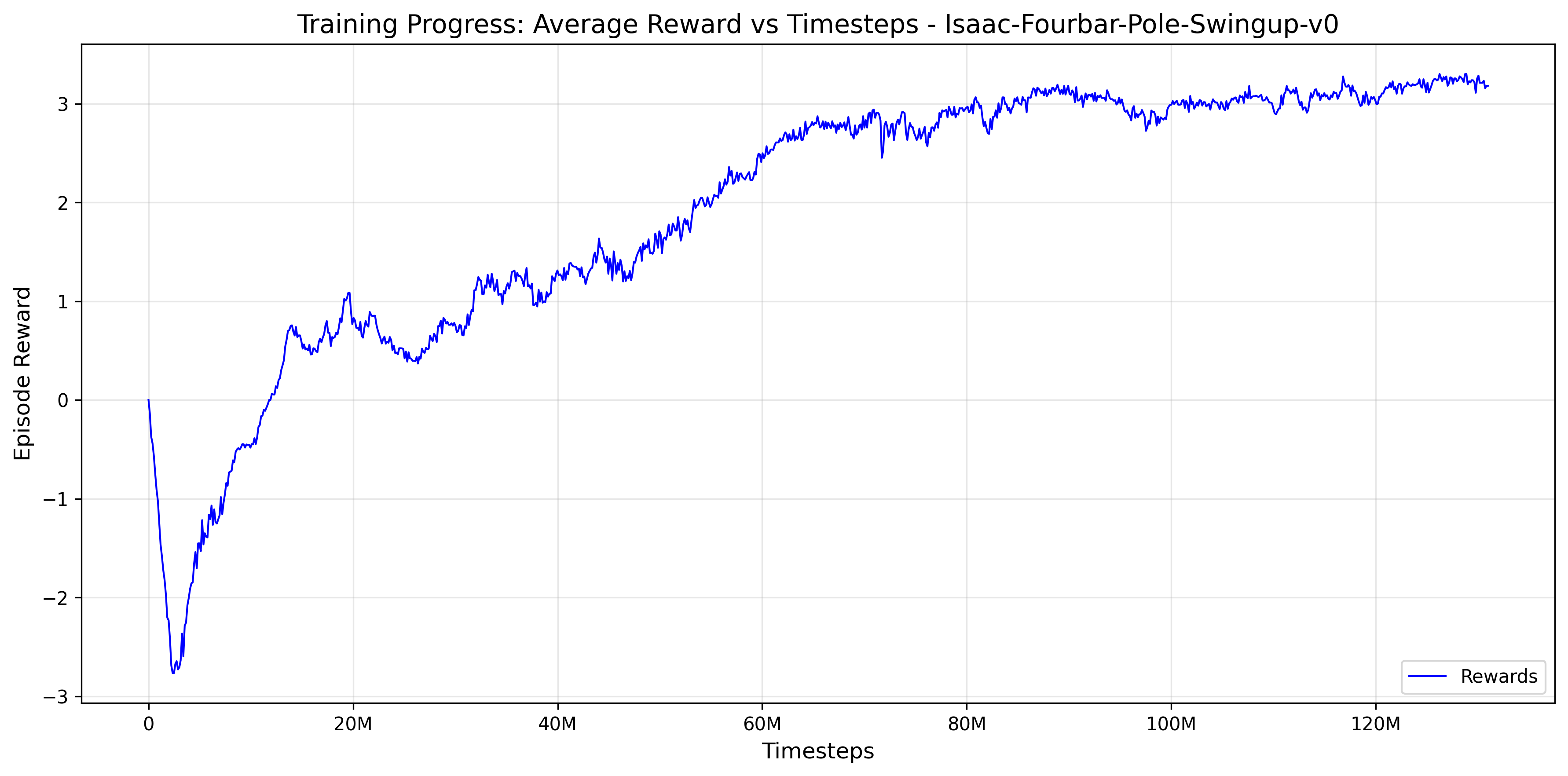
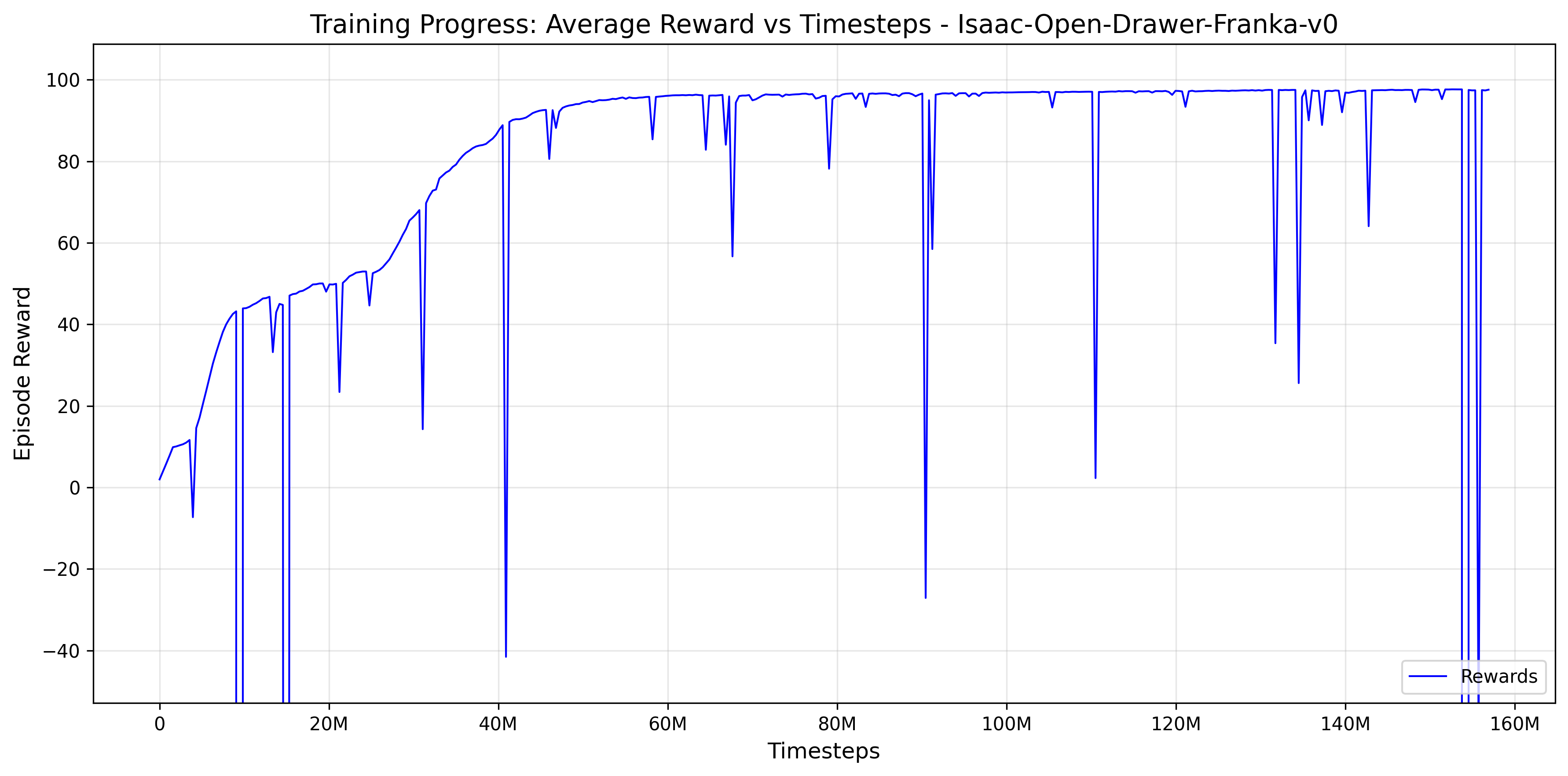
The reach task above is the one I have done sim-to-real transfer with a real SO-ARM101, which turned out to be a much harder problem than training it was. That is its own write-up.